Labelling Legal Clauses with a Simple Classification Model

A common task in legal involves identifying the types of clauses contained within a repository of contracts. This time consuming process can be automated using Machine Learning by training a classification model on a set of example clauses of different types. In this article we’ll go through some of the steps required to train a model such as the one we have deployed on on the Simplexico legal AI demo page.

Document Classification

Document classification is one of the most common tasks in Natural Language Processing. A document classification model takes a piece of text as input and assigns to it a label from a number of predefined categories. Many machine learning models can be used as document classifiers, and most recently the BERT family of language models can be fine-tuned for domain specific classification tasks. In this article we’ll show how a simple clause classification model can be constructed using packages from the well-known scikit-learn library and the open source CUAD contract dataset.

Training Data

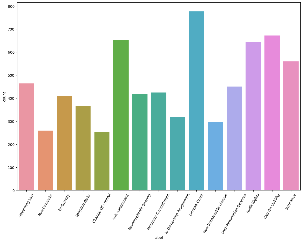
The Contract Understanding Atticus Dataset (CUAD) consists of 510 labelled contracts with 13,000+ annotations. The plot below shows the counts of the 15 most frequently labelled clauses over all contracts. We’ll extract the text from the contracts that corresponds to these annotated clauses and use them as a basis for training a classification model.

The data set consists of 9420 examples including a number of clauses with no label that we consider as belonging to a miscellaneous class labeled “null”. These examples are split into two sets for training and evaluation.

In the above code snippet X, y correspond to lists of clause text and labels respectively.

Classification Pipeline

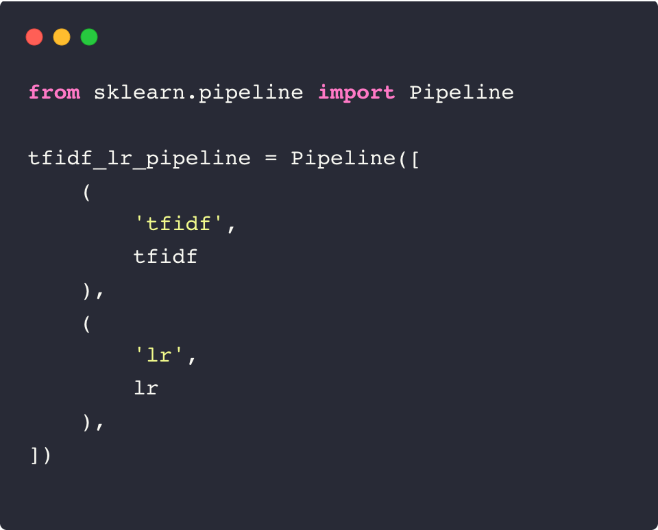
For this classification problem, we will use a simple two step model pipeline consisting of a vectorizer and a logistic regression classifier. Each of these steps will be explained below.

Vectorization

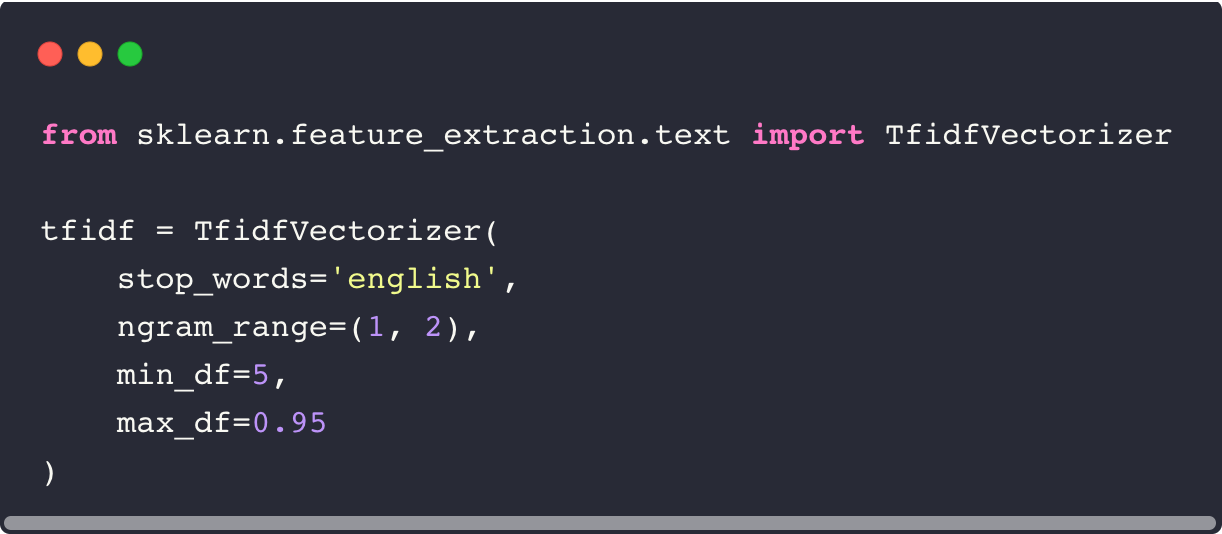
In order for textual data to be input to a machine learning algorithm, it must first be converted into a sequence of numbers, or vectorized. In this example we use a TF-IDF (term-frequency*inverse document frequency) vectorizer. For each input document, the TF-IDF vectorizer produces a vector with the number of elements equal to the number of unique terms, or dictionary, in the corpus of documents (additionally n-grams may also be included). Usually stop words (common words that do not necessarily provide much discriminative information) are subtracted from this list. For a given document each element corresponds to the number of occurrences of a given term (or n-gram) divided by the number of documents in the corpus that contain that term.

Here we specify the use of mono- and bi-grams in the vectorization and also the minimum and maximum document frequency for a term to be considered. More details about the TF-IDF vectorizer can be found here. TF-IDF vectorization produces sparse vectors of very high dimensionality, meaning that most of elements are zero for a given example document. This is in contrast to the vectors produced by embedding models such as word2vec, which produce lower dimensional dense vectors where each element is non-zero.

Model

For our classifier we have chosen the well-known logistic regression model. This model takes a linear combination of the input vector and learned weights and “squashes” them using the logistic function to produce a probability of a data point belonging to a specific class or not. Logistic regression classifiers can be trained very quickly on limited hardware.

We can combine these steps in a scikit-learn pipeline:

Training and Results

With scikit-learn we can compute the learning curve of this pipeline with respect to the training data. This gives us a sense of how the model improves as more data is added. The whole curve can be calculated on a laptop with multithreading in less than a minute.

We can plot these results:

Here we are calculating the f1-macro score which is the average of f1 scores calculated for each of our 16 classes (15 clause types and a “miscellaneous” catch-all class). We can see that the performance plateaus at around 0.7 in this case. The gap between the training and test score gives us a sense of how well the model generalizes. A large difference in score would indicate overfitting.

In this example we are not optimizing any of the model hyperparameters or performing complex preprocessing on the text. In practice we would perform an optimisation such as a grid search over a set of parameters for both the classifier and vectorizer in order to squeeze the highest possible performance from our model. Here we are limiting ourselves to a single parameter set.

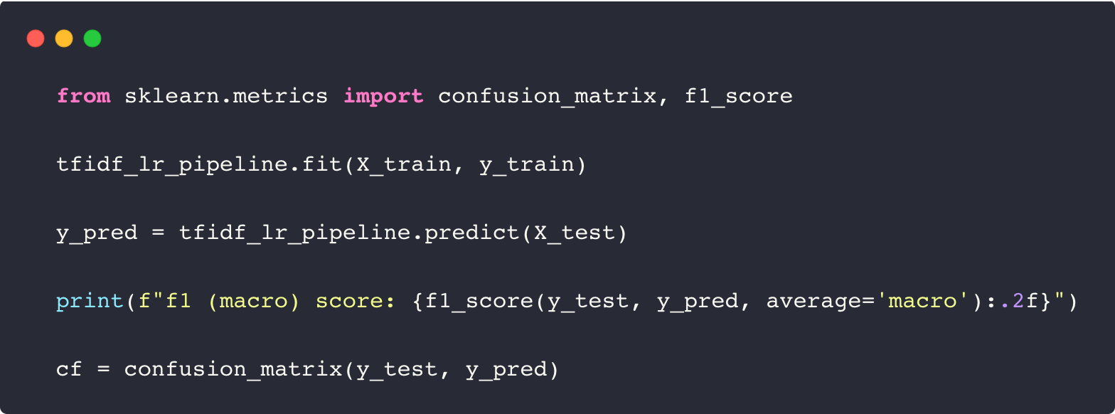
We can now train our final model on the full set of training data and evaluate on our test data:

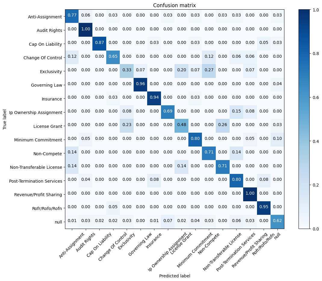
The overall score is 0.72. The confusion matrix gives a complete overview of the misclassifications in our test data.

We can see that certain classes, such as “Exclusivity” and “License Grant”, perform badly and are consistently confused with other clause types. We may be able to improve the performance on these classes with additional text processing or stemming.

Summary

We created a simple clause classification model using the CUAD open source dataset and the scikit-learn library. In this example we didn’t implement any optimisation so there should be some room for improvement! One of the advantages of this approach is that we do not need specialized hardware such as GPUs to train these models - they can be trained in a matter of seconds on a laptop and easily deployed to the cloud on services such as Amazon Sagemaker or Hugging Face.